KINEMATICS
| Site: | Newgate University Minna - Elearning Platform |
| Course: | Electrophysics I |
| Book: | KINEMATICS |
| Printed by: | Guest user |
| Date: | Monday, 8 December 2025, 3:58 PM |
Description
This course provides a fundamental understanding of motion (kinematics) and the mathematical tools used to describe it (vector algebra). Students will learn about position, velocity, and acceleration in different coordinate systems, along with vector operations essential for solving physical problems in mechanics.
1. INTRODUCTION
1.0 INTRODUCTIONKinematics is the branch of physics that describes the motion of objects without considering the forces that cause the motion. It focuses on position, displacement, velocity, acceleration, and time.
For example, a car moves on the road. Kinematics will help us understand the followings:
- How far did the car travel? (Displacement)
- How fast is the car moving? (Velocity)
- Is the car speeding up or slowing down? (Acceleration)
Instead of looking at why the car moves (like friction or engine power), kinematics only describes how it moves.
Furthermore, kinematics places more emphasis on the following's factors:- Displacement – The shortest distance from the starting point to the ending point.
- Example: If a boy run 7 meters North and 7 meters South, the displacement equal to 0 meters (because he ended up where he started).
- Velocity – The speed of an object with direction.
- Example: A car moving at 25 km/h east has a velocity of 25 km/h in the east direction.
- Acceleration – The rate of change of velocity over time.
- Example: If a car starts from rest and reaches 15 m/s in 6 seconds, its acceleration is 2 m/s².
- Time -The duration in which motion occurs.
2. VECTOR
1.1 Definition of a Vector
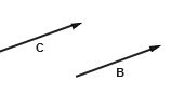
Mathematicians think of a vector as a set of numbers accompanied by rules for how they change when the coordinate system is changed. For our purposes, a down to earth geometric definition will do we can think of a vector as a directed line segment. We can represent a vector graphically by an arrow, showing both its scale length and its direction. Vectors are sometimes labelled by letters capped by an arrow, for instance A, but we shall use the convention that a bold face letter, such as A, stands for a vector.
To describe a vector, we must specify both its length and its direction. Unless indicated otherwise, we shall assume that parallel translation does not change a vector. Thus, the arrows in the sketch all represent the same vector.
![]()
3. THE ALGEBRIC OF VECTORS
1.2 The Algebra of Vectors
If two vectors have the same length and the same direction, they are equal. The vectors B = C are equal.
The magnitude or size of a vector is indicated by vertical bars or, if no confusion will occur, by using italics. For example, the magnitude of A is written |A|, or simply A. If the length of A is :2, then |A| = A = :2. Vectors can have physical dimensions, for example distance, velocity, acceleration, force, and momentum.
If the length of a vector is one unit, we call it a unit vector. A unit vector is labeled by a caret; the vector of unit length parallel to A is Aˆ . It follows that
A
Aˆ =![]()
A
and conversely
A = AAˆ .
The physical dimension of a vector is carried by its magnitude. Unit vectors are dimensionless.
1.2.1Multiplying a Vector by a Scalar
If we multiply A by a simple scalar, that is, by a simple number b, the result is a new vector C = bA. If b > 0 the vector C is parallel to A, and its magnitude is b times greater. Thus Cˆ = Aˆ , and C = bA.
If b < 0, then C = bA is opposite in direction (antiparallel) to A, and its magnitude is C = |b| A.
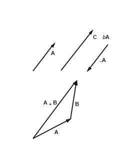
1.2.2 Adding Vectors
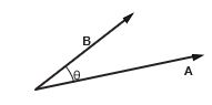
Addition of two vectors has the simple geometrical interpretation shown by the drawing. The rule is: to add B to A, place the tail of B at the head of A by parallel translation of B. The sum is a vector from the tail of A to the head of B.
1.2.3 Subtracting Vectors
Because A 2 B = A+ (2B), to subtract B from A we can simply multiply B by –1 and then add. The sketch shows how.
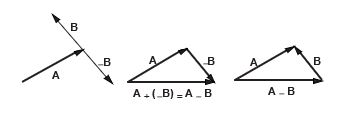
An equivalent way to construct A 2 B is to place the head of B at the head of A. Then A 2 B extends from the tail of A to the tail of B, as shown in the drawing.
1.2.4 Algebraic Properties of Vectors
It is not difficult to prove the following: Commutative law
A+B = B+A.
Associative law
A+ (B+C) = (A+B) +C c(dA) = (cd)A.
Distributive law
c(A+B) = cA+ cB
(c + d)A = cA+ dA.
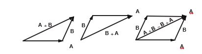
The sketch shows a geometrical proof of the commutative law A+B = B+A; try to cook up your own proofs of the others.
4. VECTOR MULTIPLICATION
1.3 Multiplying Vectors
Multiplying one vector by another could produce a vector, a scalar, or some other quantity. The choice is up to us. It turns out that two types of vector multiplication are useful in physics.
1.3.1 Scalar Product (“Dot Product”)
The first type of multiplication is called the scalar product because the result of the multiplication is a scalar. The scalar product is an operationThat combines vectors to form a scalar. The scalar product to A and B is written as A.B. Therefore often called the Dot Product (AdotB)
![]()
"Here is the angle between A and B when they are drawn tail to tail. Because Bcos" is the project of B along the direction of A. It follows that A · B = A times the projection of B on A
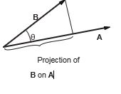
= B times the projection of A on B.
Note that A · A = |A|2 = A2. Also, A · B = B · A; the order does not change the value. We say that the dot product is commutative.
If either A or B is zero, their dot product is zero. However, because cosÃ/2 = 0 the dot product of two non-zero vectors is nevertheless zero if the vectors happen to be perpendicular.
A great deal of elementary trigonometry follows from the properties of vectors. Here is an almost trivial proof of the law of cosines using the dot product.