
4.5 Types of Search Algorithms
2. Informed Search Algorithms
The informed search algorithm is also called heuristic search or directed search. In contrast to uninformed search algorithms, informed search algorithms require details such as distance to reach the goal, steps to reach the goal, and cost of the paths, which makes this algorithm more efficient.
Here, the goal state can be achieved by using the heuristic function. The heuristic function achieves the goal state with the lowest cost possible. This function estimates how close a state is to the goal.
1. Greedy best-first search algorithm
Greedy best-first search uses the properties of both depth-first search and breadth-first search. It traverses the node by selecting the path that appears best at the moment. The closest path is selected using the heuristic function.
Consider the below graph with the heuristic values.
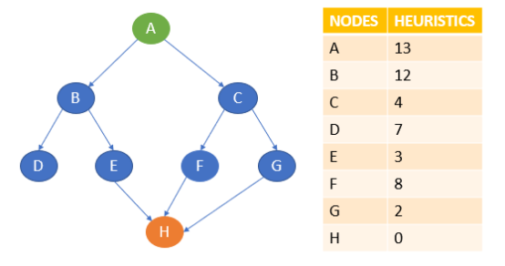
Here, A is the start node, and H is the goal node.
Greedy best-first search starts with A and then examines the next neighbours, B and C. Here, the heuristics of B are 12 and C are 4. The best path at the moment is C, so it goes to C. From C, it explores the neighbours F and G. The heuristics of F are 8 and G are 2, so it goes to G. From G, it goes to H, whose heuristic is 0, which is also our goal state.
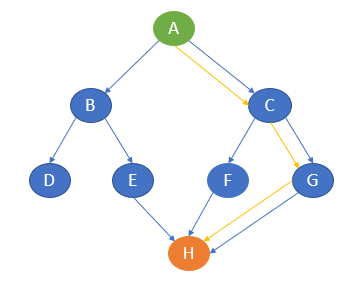
The path of traversal is
A —-> C —-> G —-> H
Let’s try this with Python.
graph = {
'A':[('B',12), ('C',4)],
'B':[('D',7), ('E',3)],
'C':[('F',8), ('G',2)],
'D':[],
'E':[('H',0)],
'F':[('H',0)],
'G':[('H',0)]
}
def bfs(start, target, graph, queue=[], visited=[]):
if start not in visited:
print(start)
visited.append(start)
queue=queue+[x for x in graph[start] if x[0][0] not in visited]
queue.sort(key=lambda x:x[1])
if queue[0][0]==target:
print(queue[0][0])
else:
processing=queue[0]
queue.remove(processing)
bfs(processing[0], target, graph, queue, visited)
bfs('A', 'H', graph)
Advantages of Greedy best-first search
- Greedy best-first search is more efficient compared with breadth-first search and depth-first search.
Disadvantages of Greedy best-first search
l In the worst-case scenario, the greedy best-first search algorithm may behave like an unguided DFS.
- There are some possibilities for greedy best-first to get trapped in an infinite loop.
- The algorithm is not an optimal one.
2. A* search Algorithm
A* search algorithm is a combination of uniform cost search and greedy best-first search algorithms. It combines the advantages of both with better memory usage. It uses a heuristic function to find the shortest path. A* search algorithm uses the sum of the node’s cost and heuristic to find the best path.
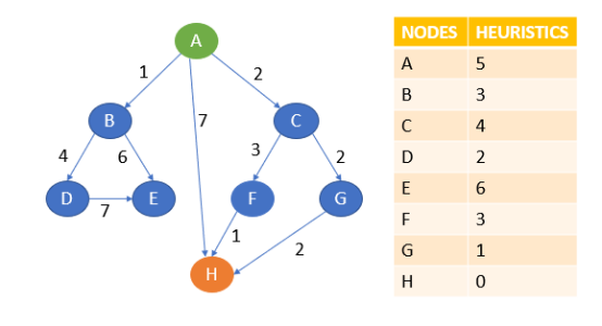
Let A be the start node, and H be the goal node.
The algorithm will start with A. From A, it can move to B, C, or H.
Note that an A* search uses the sum of path cost and heuristics value to determine the path.
Here, from A to B, the sum of cost and heuristics is 1 + 3 = 4.
From A to C, it is 2 + 4 = 6.
From A to H, it is 7 + 0 = 7.
Here, the lowest cost is 4, and the path A to B is chosen. The other paths will be on hold.
Now, from B, it can go to D or E.
The cost is 1 + 4 + 2 = 7 from A to B to D.
From A to B to E, 1 + 6 + 6 = 13.
The lowest cost is 7. Path A to B to D is chosen and compared with other on-hold paths.
Here, paths A to C are of less cost. That is 6.
Hence, A to C is chosen, and other paths are kept on hold.
From C, it can now go to F or G.
From A to C to F, the cost is 2 + 3 + 3 = 8.
The cost is 2 + 2 + 1 = 5 from A to C to G.
The lowest cost is 5, which is also less than other paths on hold. Hence, paths A to G are chosen.
From G, it can go to H, whose cost is 2 + 2 + 2 + 0 = 6.
Here, 6 is less than the cost of other paths, which is on hold.
Also, H is our goal state. The algorithm will terminate here.
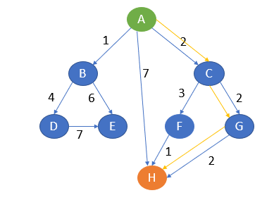
Let’s try this in Python.
graph=[['A','B',1,3],
['A','C',2,4],
['A','H',7,0],
['B','D',4,2],
['B','E',6,6],
['C','F',3,3],
['C','G',2,1],
['D','E',7,6],
['D','H',5,0],
['F','H',1,0],
['G','H',2, 0]]
temp = []
temp1 = []
for i in graph:
temp.append(i[0])
temp1.append(i[1])
nodes = set(temp).union(set(temp1))
def A_star(graph, costs, open, closed, cur_node):
if cur_node in open:
open.remove(cur_node)
closed.add(cur_node)
for i in graph:
if(i[0] == cur_node and costs[i[0]]+i[2]+i[3] < costs[i[1]]):
open.add(i[1])
costs[i[1]] = costs[i[0]]+i[2]+i[3]
path[i[1]] = path[i[0]] + ' -> ' + i[1]
costs[cur_node] = 999999
small = min(costs, key=costs.get)
if small not in closed:
A_star(graph, costs, open,closed, small)
costs = dict()
temp_cost = dict()
path = dict()
for i in nodes:
costs[i] = 999999
path[i] = ' '
open = set()
closed = set()
start_node = input("Enter the Start Node: ")
open.add(start_node)
path[start_node] = start_node
costs[start_node] = 0
A_star(graph, costs, open, closed, start_node)
goal_node = input("Enter the Goal Node: ")
print("Path with least cost is: ",path[goal_node])
Advantages of A* search algorithm
- This algorithm is best when compared with other algorithms.
- This algorithm can be used to solve very complex problems, and it is an optimal one.
Disadvantages of A* search algorithm
- The A* search is based on heuristics and cost. It may not produce the shortest path.
- Memory usage is more as it keeps all the nodes in the memory.