
4.5 Types of Search Algorithms
1. Uninformed Search Algorithms
Based on the search problems, we can classify the search algorithm as:
- Uninformed search
- Informed search
Uninformed Search Algorithms
The uninformed search algorithm does not have any domain knowledge, such as closeness, location of the goal state, etc. It behaves in a brute-force way. It only knows how to traverse the given tree and find the goal state. This algorithm is also known as the Blind search algorithm or brute-force algorithm. There are six types of uninformed search strategies. They are:
- Breadth-first search
- Depth-first search
- Depth-limited search
- Iterative deepening depth-first search
- Bidirectional search
- Uniform cost search
1. Breadth-first search
It is one of the most common search strategies. A breadth-first search generally starts from the root node, examines the neighbor nodes, and then moves to the next level. It uses the First-in, First-out (FIFO) strategy as it gives the shortest path to achieving the solution. BFS is used where the given problem is very small and space complexity is not considered. Now, consider the following tree.
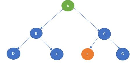
Let’s take node A as the start state and node F as the goal state.
The BFS algorithm starts with the start state, moves to the next level, and visits each node until it reaches the goal state.
In this example, it starts from A and then travels to the next level and visits B and C and then. Travel to the next level and visit D, E, F, and G. Here, the goal state is defined as F, so the traversal will stop at F.
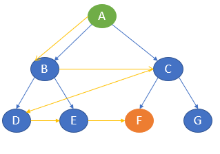
The path of traversal is:
A —-> B —-> C —-> D —-> E —-> F
Let’s implement the same in Python programming.
Python Code:
graph = {
'A' : ['B','C'],
'B' : ['D', 'E'],
'C' : ['F', 'G'],
'D' : [],
'E' : [],
'F' : [],
'G' : []
}
visited = []
queue = []
goal = 'F'
def bfs(visited, graph, node):
visited.append(node)
queue.append(node)
while queue:
s = queue.pop(0)
print (s, end = "\n")
for neighbour in graph[s]:
if neighbour not in visited:
visited.append(neighbour)
queue.append(neighbour)
if goal in visited:
break
bfs(visited, graph, 'A')
Advantages of BFS
- BFS will never be trapped in any unwanted nodes.
- If the graph has more than one solution, then BFS will return the optimal solution with the shortest path.
Disadvantages of BFS
- BFS stores all the nodes in the current level and then moves them to the next level. This requires a lot of memory.
- BFS takes more time to reach the goal state, which is far away.
2. Depth-first search
The depth-first search uses Last-in, First-out (LIFO) strategy and hence it can be implemented by using stack. DFS uses backtracking. It starts from the initial state and explores each path to its greatest depth before it moves to the next path.
DFS will follow
Root node —-> Left node —-> Right node
Now, consider the same example tree mentioned above.
Here, it starts from the start state A, then travels to B, then goes to D. After reaching D, it backtracks to B. B is already visited, so it goes to the next depth, E, and then backtracks to B. As it is already visited, it goes back to A. A is already visited, so it goes to C and then to F. F is our goal state, and it stops there.
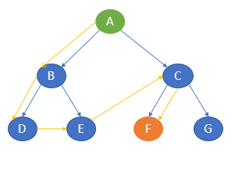
The path of traversal is:
A —-> B —-> D —-> E —-> C —-> F
Let’s try to code it.
graph = {
'A' : ['B','C'],
'B' : ['D', 'E'],
'C' : ['F', 'G'],
'D' : [],
'E' : [],
'F' : [],
'G' : []
}
goal = 'F'
visited = set()
def dfs(visited, graph, node):
if node not in visited:
print (node)
visited.add(node)
for neighbour in graph[node]:
if goal in visited:
break
else:
dfs(visited, graph, neighbour)
dfs(visited, graph, 'A')
Advantages of DFS
- It takes lesser memory as compared to BFS.
- The time complexity is lesser when compared to BFS.
- DFS does not require much more search.
Disadvantages of DFS
- DFS does not always guarantee to give a solution.
- As DFS goes deep down, it may get trapped in an infinite loop.
3. Depth-limited search
Depth-limited search works similarly to depth-first search. The difference is that depth-limited search has a pre-defined limit up to which it can traverse the nodes. Depth-limited search solves one of DFS’s drawbacks, as it does not go to an infinite path.
DLS ends its traversal if any of the following conditions exits.
- Standard Failure
- It denotes that the given problem does not have any solutions.
- Cut off Failure Value
- It indicates no solution for the problem within the given limit.
Now, consider the same example.
Let’s take A as the start node and C as the goal state and limit as 1.
The traversal starts with node A and then goes to the next level, 1. The goal state C is there, and it stops the traversal.
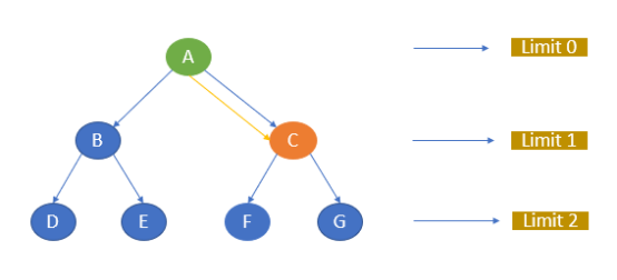
The path of traversal is:
A —-> C
If we give C as the goal node and the limit as 0, the algorithm will not return any path as the goal node is unavailable within the given limit.
If we give the goal node as F and the limit as 2, the path will be A, C, F.
Let’s implement DLS.
graph = {
'A' : ['B','C'],
'B' : ['D', 'E'],
'C' : ['F', 'G'],
'D' : [],
'E' : [],
'F' : [],
'G' : []
}
def DLS(start,goal,path,level,maxD):
print('nCurrent level-->',level)
path.append(start)
if start == goal:
print("Goal test successful")
return path
print('Goal node testing failed')
if level==maxD:
return False
print('nExpanding the current node',start)
for child in graph[start]:
if DLS(child,goal,path,level+1,maxD):
return path
path.pop()
return False
start = 'A'
goal = input('Enter the goal node:-')
maxD = int(input("Enter the maximum depth limit:-"))
print()
path = list()
res = DLS(start,goal,path,0,maxD)
if(res):
print("Path to goal node available")
print("Path",path)
else:
print("No path available for the goal node in given depth limit")
Advantages of DLS
- It takes lesser memory when compared to other search techniques.
Disadvantages of DLS
- DLS may not offer an optimal solution if the problem has multiple solutions.
- DLS also encounters incompleteness.
4. Iterative deepening depth-first search
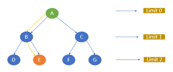
Iterative deepening depth-first search is a combination of depth-first search and breadth-first search. IDDFS find the best depth limit by gradually adding the limit until the defined goal state is reached.
Let me try to explain this using the same example tree.
Consider A as the start node and E as the goal node. Let the maximum depth be 2.
The algorithm starts with A, moves to the next level, and searches for E. If it does not find E, it moves to the next level and finds it again.
The path of traversal is
A —-> B —-> E
Let’s try to implement this.
graph = {
'A' : ['B','C'],
'B' : ['D', 'E'],
'C' : ['F', 'G'],
'D' : [],
'E' : [],
'F' : [],
'G' : []
}
path = list()
def DFS(currentNode,destination,graph,maxDepth,curList):
curList.append(currentNode)
if currentNode==destination:
return True
if maxDepth<=0:
path.append(curList)
return False
for node in graph[currentNode]:
if DFS(node,destination,graph,maxDepth-1,curList):
return True
else:
curList.pop()
return False
def iterativeDDFS(currentNode,destination,graph,maxDepth):
for i in range(maxDepth):
curList = list()
if DFS(currentNode,destination,graph,i,curList):
return True
return False
if not iterativeDDFS('A','E',graph,3):
print("Path is not available")
else:
print("Path exists")
print(path.pop())
Advantages of IDDFS
- IDDFS has the advantages of both BFS and DFS.
- It offers fast search and uses memory efficiently.
Disadvantages of IDDFS
- It does all the work of the previous stage again and again.
5. Bidirectional search
The bidirectional search algorithm is completely different from all other search strategies. It executes two simultaneous searches called forward and backward searches and reaches the goal state. Here, the graph is divided into two smaller sub-graphs. In one graph, the search is started from the initial start state, and in the other graph, it is started from the goal state. When these two nodes intersect, the search will be terminated.
Bidirectional search requires the well-definition of both the start and goal start and the same branching factor in both directions. Consider the graph below.
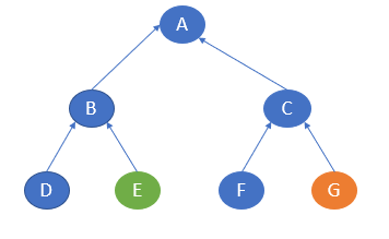
Here, the start state is E, and the goal state is G. In one sub-graph, the search starts from E, and in the other, it starts from G. E will go to B and then A, and G will go to C and then A. Here, both traversals meet at A, and hence, the traversal ends.
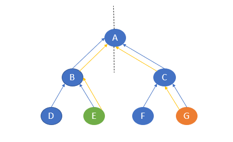
The path of traversal is
E —-> B —-> A —-> C —-> G
Let’s implement the same in Python.
from collections import deque
class Node:
def __init__(self, val, neighbors=[]):
self.val = val
self.neighbors = neighbors
self.visited_right = False
self.visited_left = False
self.parent_right = None
self.parent_left = None
def bidirectional_search(s, t):
def extract_path(node):
node_copy = node
path = []
while node:
path.append(node.val)
node = node.parent_right
path.reverse()
del path[-1]
while node_copy:
path.append(node_copy.val)
node_copy = node_copy.parent_left
return path
q = deque([])
q.append(s)
q.append(t)
s.visited_right = True
t.visited_left = True
while len(q) > 0:
n = q.pop()
if n.visited_left and n.visited_right:
return extract_path(n)
for node in n.neighbors:
if n.visited_left == True and not node.visited_left:
node.parent_left = n
node.visited_left = True
q.append(node)
if n.visited_right == True and not node.visited_right:
node.parent_right = n
node.visited_right = True
q.append(node)
return False
n0 = Node('A')
n1 = Node('B')
n2 = Node('C')
n3 = Node('D')
n4 = Node('E')
n5 = Node('F')
n6 = Node('G')
n0.neighbors = []
n1.neighbors = [n0]
n2.neighbors = [n0]
n3.neighbors = [n1]
n4.neighbors = [n1]
n5.neighbors = [n2]
n6.neighbors = [n2]
print(bidirectional_search(n4, n6))
Advantages of bidirectional search
- This algorithm searches the graph fast.
- It requires less memory to complete its action.
Disadvantages of bidirectional search
- The goal state should be pre-defined.
- The graph is quite difficult to implement.
6. Uniform cost search
Uniform cost search is considered the best search algorithm for a weighted graph or graph with costs. It searches the graph by giving maximum priority to the lowest cumulative cost. Uniform cost search can be implemented using a priority queue.
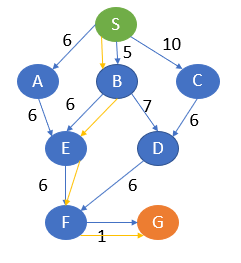
Consider the below graph where each node has a pre-defined cost.
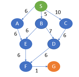
Here, S is the start node and G is the goal node.
From S, G can be reached in the following ways.
S, A, E, F, G -> 19
S, B, E, F, G -> 18
S, B, D, F, G -> 19
S, C, D, F, G -> 23
Here, the path with the least cost is S, B, E, F, G.
Let’s implement UCS in Python.
graph=[['S','A',6],
['S','B',5],
['S','C',10],
['A','E',6],
['B','E',6],
['B','D',7],
['C','D',6],
['E','F',6],
['D','F',6],
['F','G',1]]
temp = []
temp1 = []
for i in graph:
temp.append(i[0])
temp1.append(i[1])
nodes = set(temp).union(set(temp1))
def UCS(graph, costs, open, closed, cur_node):
if cur_node in open:
open.remove(cur_node)
closed.add(cur_node)
for i in graph:
if(i[0] == cur_node and costs[i[0]]+i[2] < costs[i[1]]):
open.add(i[1])
costs[i[1]] = costs[i[0]]+i[2]
path[i[1]] = path[i[0]] + ' -> ' + i[1]
costs[cur_node] = 999999
small = min(costs, key=costs.get)
if small not in closed:
UCS(graph, costs, open,closed, small)
costs = dict()
temp_cost = dict()
path = dict()
for i in nodes:
costs[i] = 999999
path[i] = ' '
open = set()
closed = set()
start_node = input("Enter the Start State: ")
open.add(start_node)
path[start_node] = start_node
costs[start_node] = 0
UCS(graph, costs, open, closed, start_node)
goal_node = input("Enter the Goal State: ")
print("Path with least cost is: ",path[goal_node])
Advantages of UCS
- This algorithm is optimal as the selection of paths is based on the lowest cost.
Disadvantages of UCS
- The algorithm does not consider how many steps it takes to reach the lowest path. This may result in an infinite loop also.